© 2018 *All rights reserved by liudx .:smile:
Python的matplotlib是一个功能强大的绘图库,可以很方便的绘制数学图形。官方给出了很多简单的实例,结合中文翻译的示例Tutorial,可以满足日常工作的大部分需求了。但是实际工作中,一些有趣的东西很难使用常规方程(笛卡尔坐标和极坐标)方式绘制,事实上,大部分工程上都是使用参数方程来描述曲线。本文给出一些参数方程绘制的实例,之后会扩展为动画形式绘制,可以看到这些复杂的方程是如何简单优美的绘制出来。
1 参数方程绘制
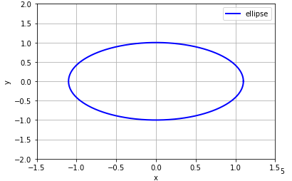
首先介绍下椭圆的参数方程:
$$
\begin{cases}
x = a \cdot \cos(t)\\
y = b \cdot \sin(t)
\end{cases}
$$
其中$a,b$分别是椭圆的长轴、短轴。绘制椭圆的python代码如下:
1 | import matplotlib.pyplot as plt |
结果如下:
下面我们来个复杂点的例子,绘制炮弹的弹道曲线(当然是理想情况的),我们先根据公式推算一把,首先我们设炮弹出口速度$v_0(m/s)$,向上仰角为$\theta$ °,时间为$t(s)$, 大炮的筒口初始坐标初始为(0,0),则有:
$$
\begin{cases}
x=v_0\cdot\sin(\theta)\cdot t \\
y=v_0\cdot\cos(\theta)\cdot t - v_0\cdot\cos(\theta)\cdot g \cdot t^2
\end{cases}
$$
对应python代码為:
1 | def Parabolic(v0, theta_x): # 模拟炮弹飞行曲线 |
为了方便示意,我分别绘制了初速为$100m/s$时,仰角为45°、30°、60°的炮弹落地曲线:
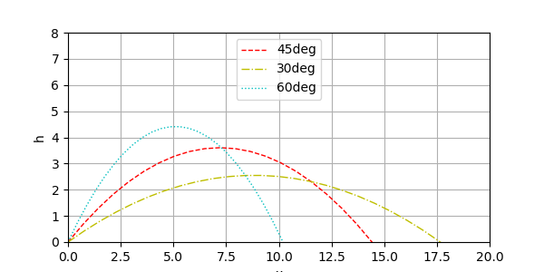
验证了我们高中物理中的一个结论:这货不就是抛物线嘛。
2 动画animation
看完静态的参数方程,还是不过瘾,我们来做个动画玩玩。首先是绘制一个内旋轮,引用下这位老哥的例子:
1 | import numpy as np |
看起来很不错,能动(这里发现了init函数可以绘制下静态的大圆ln1,update函数只对动圆ln2的plot对象数据进行更新):
最后研究下旋轮线, 看看能否绘制出wiki页面上那个动画效果。先列出参数方程:
$$
选轮线参数方程:
\begin{cases}
x = r\cdot(t-\sin t) \\
y = r \cdot (1-\cos t)
\end{cases}
\\
圆心的坐标为:(t,r)
$$
经过观察摸索,发现需要绘制3部分,一个是滚动的圆,一个是摆线,还有个圆心到绘制曲线的支点。坐标都可直接从参数方程推算出来,不多说,直接上代码和注释吧:
1 | #def wheel_line(): |
大功告成:
3 后记
在摸索过程中,还是有很多坑需要注意的,最初那个摆线的例子,我没有计算好图形范围,画出来的圆是扁扁的,后来通过改figsize和ax.set_xlim/set_ylim为相同比例解决的;保存动画那个ani.save('roll.gif', writer='imagemagick', fps=60)总是报错,经过查找资料,解决方案是安装imagemagic,下载安装后第2节的例子都能顺利保存动图为gif。还有需要注意是的save函数里面的fps参数不能调太低,否则会出现动画卡顿的现象,太高又会出现动画速度很快的问题,这个参数需要配合frames即动画的总帧数,以及FuncAnimation里面的interval帧间隔时间参数(单位是ms),总动画时间(秒)公式为:$frames * interval/1000+frames/fps$。
读完这篇文章,相信绘制参数方程和动画不是一件难事吧:smile:。